Flow and bottleneck game

This game simulates the flow of items between workstations and can be used to demonstrate a number of Lean flow and variation principles. The basic set-up is to have a number of “workstations” (these could also represent teams or single workers) in a chain. Items are added to one end of the chain and output at the other. Each workstation uses dice to decide how many items are processed (the throwing of the dice simulating random variation within the limits of 1 - 6). The number of outputs is recorded over a number of cycles.

Here’s how to play the game – you’ll need 4 or 5 workstations (i.e. 4 or 5 people), plus a customer and a monitor, so 6 or 7 people overall. You can have multiple “teams” if you want to run this with several groups. (In fact this is interesting in itself as you can then simulate team performance across different teams).

Each workstation has an in-box, which is where incoming items/tasks are stored and a processing unit which is the person throwing a dice to see how many items they can process and pass along the chain. At the beginning of the simulation the workstations each have 3 items in their in boxes.

You can use coloured card, tiddly-wink counters, etc. to represent the work items. You’ll need a stock of these to run the simulation – maximum 120 for a 20 cycle run.

The customer introduces new work items to the chain and the monitor records the output for each cycle.
So a typical set-up is as shown below.

The rules are as follows:

1. At the beginning of each cycle everyone throws their dice and “processes” their inbox accordingly (before anything is added).
2. Each workstation passes on the number of items according to their dice throw.
3. If there are fewer items in their inbox than the number thrown they simply transfer what they have and no more.
4. Each workstation cannot wait for the preceding one to complete their transfer before doing their own transfer (as per rule 1).
5. At the end of each cycle the monitor records the number of items processed (i.e. what comes out of the end of the chain).

Let’s take an example:

On cycle 1 the customer throws a 4, A throws a 4, B throws a 3, C throws a 4, D throws a 6. A can only move 3 items to B even though they rolled a 4.  Once they have moved their items, the customer’s 4 items are added to A’s inbox. So at the end of the cycle A now has 4 items. B moves their 3 items to D and then gets three items from A, so ends up with 3 items. C, like A moves 3 items over even though they threw a 4, and then gets 3 items from B so ends up with 3. Similarly D can only transfer 3 items even though a 6 was thrown, and they too receive 3 items. The monitor records a first cycle output of 3. So we end up with…

A = 4, B = 3, C = 3, D = 3, cycle output = 3

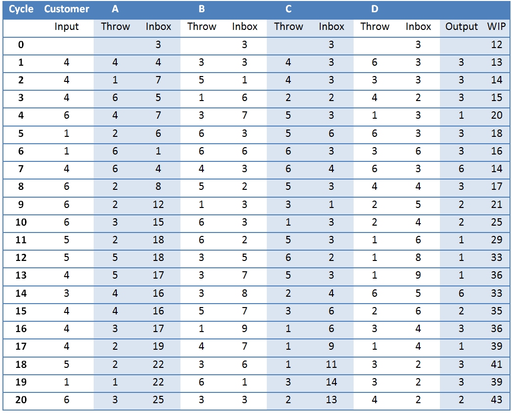
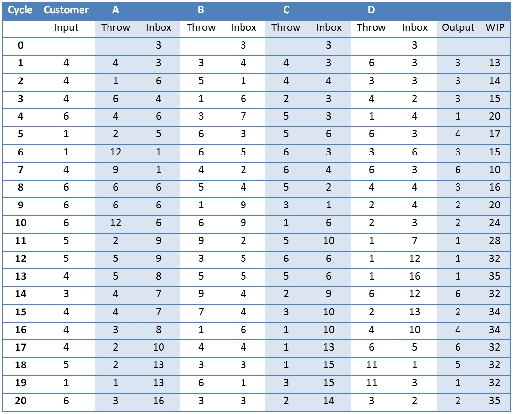
We continue in this fashion for 20 cycles. The table above (click to enlarge) shows an example (the dice throws were simulated using Excel’s randbetween function, but in the exercise real dice throws are used.

The last column in the table, WIP, is the total amount of work in progress for that cycle. We started with 12 and ended with 43, so obviously the system is not terribly efficient because if it were you’d expect the WIP to stay fairly constant.

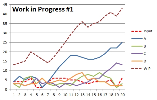
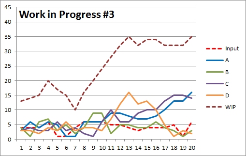
If we plot the WIP data and the input for each cycle we get a chart like the one shown here (click to enlarge). You can see that the total WIP line is steadily increasing!

Let’s now imagine management look at this pattern and decide workstation A is a problem because they don’t seem to be processing as efficiently as everyone else. In fact they might have looked at the data after the first week (i.e. cycle 5) and used a measure such as average WIP. For the four workstations, the average WIP after 5 cycles is

A =  5.4, B = 4.8, C = 4.4, D = 3.6

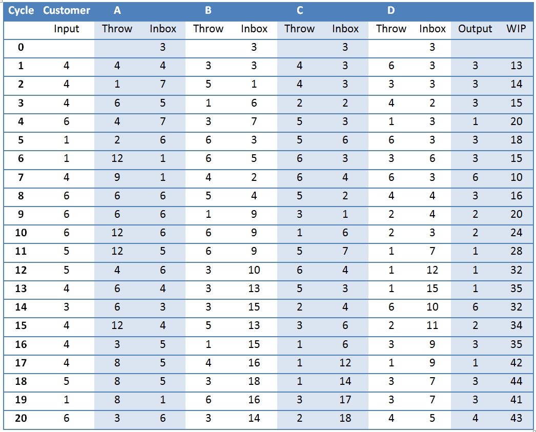
So they decide to add extra resource (another dice) to the least “efficient” workstation: A. We now run another 15 cycles, starting off from where we left off and the dice throws as shown in the able below (exactly the same as above except that A’s throws are now randomised for 2 dice, i.e. between 2 and 12).

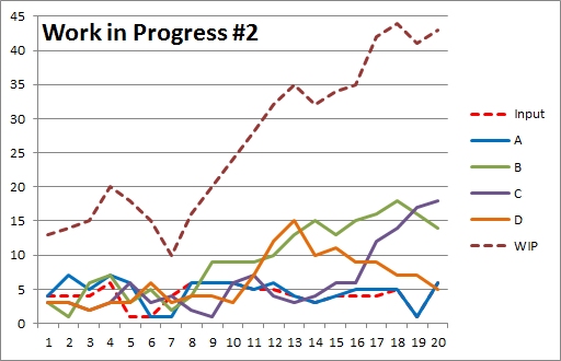
Something very odd seems to be happening: the amount of WIP doesn’t appear to have diminished at all! For the cost of extra resource there has been no improvement. The chart shows this too:

The point here is that – like all batch and queue systems, of which this is a simplified example – there is no real flow. In Lean terms the system would work on a pull basis, so would react to customer demand. So on cycle 2, after 4 items were introduced in cycle 1, the throughput at each workstation ought to be 4, and on cycle 6 the throughput needs to increase top 6 items per workstation. In this way the flow through the system reacts to customer demand and you don’t get queues forming.

So how might management react? Well if you’re lucky they’ll be a bit more finessed than the second scenario above and say they’ll move the extra resource around. The third scenario, below, uses a weekly review with the additional resource being moved to the “worst” workstation at the end of each week. It does appear to make some difference as the WIP does seem to have been reduced – though not by a huge amount.

But apart from this small improvement, the tactic doesn’t seem to have worked. Yet this is the sort of thing management usually do! And then they look for someone to blame when there is no, or little, improvement!

This little experiment is a great way of demonstrating that you can’t fix processes in that way and what you need to do is understand customer demand and then set up systems that can react to that effectively.